Accessing and analysing the OpenAIRE Research Graph data dumps
Najko Jahn
State and University Library Göttingenoaire_graph_post.RmdThe OpenAIRE Research Graph provides a wide range of metadata about grant-supported research publications. This blog post presents an experimental R package with helpers for splitting, de-compressing and parsing the underlying data dumps. I will demonstrate how to use them by examining the compliance of funded projects with the open access mandate in Horizon 2020.
OpenAIRE has collected and interlinked scholarly data from various openly available sources for over ten years. In December 2019, this open science network released the OpenAIRE Research Graph (Manghi, Atzori, et al. 2019), a big scholarly data dump that contains metadata about more than 100 million research publications and 8 million datasets, as well as the relationships between them. These metadata are furthermore connected to open access locations and disambiguate information about persons, organisations and funders.
Like most big scholarly data dumps, the OpenAIRE Research Graph offers many data analytics opportunities, but working with it is challenging. One reason is the size of the dump. Although the OpenAIRE Research Graph is already split into several files, most of these data files are too large to fit the memory of a moderately equipped laptop, when directly imported into computing environments like R. Another challenge is the format. The dump consists of compressed XML-files following the comprehensive OpenAIRE data model (Manghi, Bardi, et al. 2019), from which only certain elements may be needed for a specific data analysis.
In this blog post, I introduce the R package {openairegraph}, an experimental effort, that helps to transform the large OpenAIRE Research Graph dumps into relevant small datasets for analysis. These tools aim at data analysts and researchers alike who wish to conduct their own analysis using the OpenAIRE Research Graph, but are wary of handling its large data dumps. Focusing on grant-supported research results from the European Commission’s Horizon 2020 framework programme (H2020), I present how to subset and analyse the graph using this {openairegraph}. My analytical use case is to benchmark the open access activities of grant-supported projects affiliated with the University of Göttingen against the overall uptake across the H2020 funding activities.
What is the R package {openairegraph} about?
So far, the R package {openairegraph}, which is available on GitHub as a development version, has two sets of functions. The first set provides helpers to split a large OpenAIRE Research Graph data dump into separate, de-coded XML records that can be stored individually. The other set consists of parsers that convert data from these XML files to a table-like representation following the tidyverse philosophy, a popular approach and toolset for doing data analysis with R (Wickham et al. 2019). Splitting, de-coding and parsing are essential steps before analysing the OpenAIRE Research Graph.
Installation
openairegraph can be installed from GitHub using the remotes (Hester et al. 2019) package:
library(remotes)
remotes::install_github("subugoe/openairegraph")
Loading a dump into R
Several dumps from the OpenAIRE Research Graph are available on Zenodo (Manghi, Atzori, et al. 2019). So far, I tested openairegraph to work with the dump h2020_results.gz, which comprises research outputs funded by the European Commission’s Horizon 2020 funding programme (H2020).
After downloading it, the file can be imported into R using the jsonlite package (Ooms 2014). The following example shows that each line contains a record identifier and the corresponding Base64-encoded XML file. Base64 is a standard that allows file compression in a text-based format.
library(jsonlite) # tools to work with json files
library(tidyverse) # tools from the tidyverse useful for data analysis
# download the file from Zenodo and store it locally
dir.create("data")
download.file(
  url = "https://zenodo.org/record/3516918/files/h2020_results.gz",
  destfile = "data/h2020_results.gz"
)
oaire <- jsonlite::stream_in(file("data/h2020_results.gz"), verbose = FALSE) %>%
  tibble::as_tibble()
oaire
#> # A tibble: 92,218 x 2
#>    `_id`$`$oid`        body$`$binary`                                   $`$type`
#>    <chr>               <chr>                                            <chr>
#>  1 5dbc22f81e82127b58… UEsDBBQACAgIAIRiYU8AAAAAAAAAAAAAAAAEAAAAYm9kee1… 00
#>  2 5dbc22f9b531c546e8… UEsDBBQACAgIAIRiYU8AAAAAAAAAAAAAAAAEAAAAYm9kee0… 00
#>  3 5dbc22fa45e3122d97… UEsDBBQACAgIAIViYU8AAAAAAAAAAAAAAAAEAAAAYm9kee1… 00
#>  4 5dbc22fa45e3122d97… UEsDBBQACAgIAIViYU8AAAAAAAAAAAAAAAAEAAAAYm9kee1… 00
#>  5 5dbc22fa4e0c061a4d… UEsDBBQACAgIAIViYU8AAAAAAAAAAAAAAAAEAAAAYm9kee1… 00
#>  6 5dbc22fb81f3c12c00… UEsDBBQACAgIAIViYU8AAAAAAAAAAAAAAAAEAAAAYm9kee1… 00
#>  7 5dbc22fb895be12461… UEsDBBQACAgIAIViYU8AAAAAAAAAAAAAAAAEAAAAYm9kee2… 00
#>  8 5dbc22fbe56570673e… UEsDBBQACAgIAIViYU8AAAAAAAAAAAAAAAAEAAAAYm9kee1… 00
#>  9 5dbc22fc81f3c12bfe… UEsDBBQACAgIAIViYU8AAAAAAAAAAAAAAAAEAAAAYm9kee1… 00
#> 10 5dbc22fcb531c546e8… UEsDBBQACAgIAIZiYU8AAAAAAAAAAAAAAAAEAAAAYm9kee1… 00
#> # … with 92,208 more rows
De-coding and storing OpenAIRE Research Graph records
The function openairegraph::oarg_decode() splits and de-codes each record. Storing the records individually allows to process the files independent from each other, which is a common approach when working with big data.
library(openairegraph)
dir.create("data/records")
oarg_decode(oaire, records_path = "data/records/", limit = 500, verbose = FALSE)
openairegraph::oarg_decode() writes out each XML-formatted record as a zip file to a specified folder. Because the dumps are quite large, the function furthermore has a parameter that allows setting a limit, which is helpful for inspecting the output first. By default, a progress bar presents the current state of the process.
Parsing OpenAIRE Research Graph records
So far, there are four parsers available to consume the H2020 results set:
-
openairegraph::oarg_publications_md()retrieves basic publication metadata complemented by author details and access status -
openairegraph::oarg_linked_projects()parses grants linked to publications -
openairegraph::oarg_linked_ftxt()gives full-text links including access information -
openairegraph::oarg_linked_affiliations()parses affiliation data
These parsers can be used alone, or together like this:
First, I obtain the locations of the de-coded XML records.
openaire_records <- list.files("data/records", full.names = TRUE)
After that, I read each XML file using the xml2 (Wickham, Hester, and Ooms 2019) package, and apply three parsers: openairegraph::oarg_publications_md(), openairegraph::oarg_linked_projects() and openairegraph::oarg_linked_ftxt(). I use the future (Bengtsson 2020b) and future.apply (Bengtsson 2020a) packages to enable reading and parsing these records simultaneously with multiple R sessions. Running code in parallel reduces the execution time.
library(xml2) # working with xml files
library(future) # parallel computing
library(future.apply) # functional programming with parallel computing
library(tictoc) # timing functions

openaire_records <- list.files("data/records", full.names = TRUE)

if (!identical(Sys.getenv("GITHUB_ACTIONS"), "true")) {
  future::plan(multisession)
  tic()
  oaire_data <- future.apply::future_lapply(openaire_records, function(files) {
    # load xml file
    doc <- xml2::read_xml(files)
    # parser
    out <- oarg_publications_md(doc)
    out$linked_projects <- list(oarg_linked_projects(doc))
    out$linked_ftxt <- list(oarg_linked_ftxt(doc))
    # use file path as id
    out$id <- files
    out
  })
  toc()
} else {
  oaire_data <- lapply(openaire_records, function(files) {
    # load xml file
    doc <- xml2::read_xml(files)
    # parser
    out <- oarg_publications_md(doc)
    out$linked_projects <- list(oarg_linked_projects(doc))
    out$linked_ftxt <- list(oarg_linked_ftxt(doc))
    # use file path as id
    out$id <- files
    out
  })
}
oaire_df <- dplyr::bind_rows(oaire_data)
A note on performance: Parsing the whole dump h2020_results using these parsers took me around 2 hours on my MacBook Pro (Early 2015, 2,9 GHz Intel Core i5, 8GB RAM, 256 SSD).
I therefore recommend to back up the resulting data, instead of un-packing the whole dump for each analysis. jsonlite::stream_out() outputs the data frame to a text-based json-file, where list-columns are preserved per row.
jsonlite::stream_out(oaire_df, file("data/h2020_parsed_short.json"))
#>
Processed 500 rows...
Complete! Processed total of 500 rows.
download.file(
  url = "https://github.com/subugoe/scholcomm_analytics/releases/download/oaire_graph_post/h2020_parsed.json.gz",
  destfile = "data/h2020_parsed.json.gz"
)
oaire_df <- jsonlite::stream_in(
  file("data/h2020_parsed.json.gz"),
  verbose = FALSE
) %>%
  tibble::as_tibble()
Use case: Monitoring the Open Access Compliance across H2020 grant-supported projects at the institutional level
Usually, it is not individual researchers who sign grant agreements with the European Commission (EC), but the institution they are affiliated with. Universities and other research institutions hosting EC-funded projects are therefore looking for ways to monitor the insitutions’s overall compliance with funder rules. In the case of the open access mandate in Horizon 2020 (H2020), librarians are often assigned this task. Moreover, quantitative science studies have started to investigate the efficacy of funders’ open-access mandates. (Larivière and Sugimoto 2018)
In this use case, I will illustrate how to make use of the OpenAIRE Research Graph, which links grants to publications and open access full-texts, to benchmark compliance with the open access mandate against other H2020 funding activities.
Overview
As a start, I load a dataset, which was compiled following the above-described methods using the whole h2020_results.gz dump.
It contains 92,218 grant-supported research outputs. Here, I will focus on the prevalence of open access across H2020 projects using metadata about the open access status of a publication and related project information stored in the list-column linked_projects.
pubs_projects <- oaire_df %>%
  filter(type == "publication") %>%
  select(id, type, best_access_right, linked_projects) %>%
  # transform to a regular data frame with a row for each project
  unnest(linked_projects)
The dataset contains 84,781 literature publications from 9,008 H2020 projects. What H2020 funding activity published most?
library(cowplot)
library(scales)
pubs_projects %>%
  filter(funding_level_0 == "H2020") %>%
  mutate(funding_scheme = fct_infreq(funding_level_1)) %>%
  group_by(funding_scheme) %>%
  summarise(n = n_distinct(id)) %>%
  mutate(funding_fct = fct_other(funding_scheme, keep = levels(funding_scheme)[1:10])) %>%
  mutate(highlight = ifelse(funding_scheme %in% c("ERC", "RIA"), "yes", "no")) %>%
  ggplot(aes(reorder(funding_fct, n), n, fill = highlight)) +
  geom_bar(stat = "identity") +
  coord_flip() +
  scale_fill_manual(
    values = c("#B0B0B0D0", "#56B4E9D0"),
    name = NULL) +
  scale_y_continuous(
    labels = scales::number_format(big.mark = ","),
    expand = expansion(mult = c(0, 0.05)),
    breaks =  scales::extended_breaks()(0:25000)
    ) +
  labs(x = NULL, y = "Publications", caption = "Data: OpenAIRE Research Graph") +
  theme_minimal_vgrid() +
  theme(legend.position = "none")
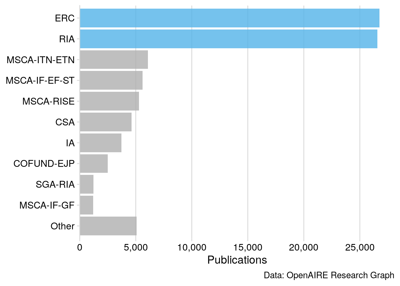
Figure 1: Publication Output of Horizon 2020 funding activities captured by the OpenAIRE Research Graph, released in December 2019.
Figure 1 shows that most publications in the OpenAIRE Research Graph originate from the European Research Council (ERC), Research and Innovation Actions (RIA) and Marie Skłodowska-Curie Actions (MSCA). On average, 10 articles were published per project. However, the publication performance per H2020 funding activity varies considerably (SD = 33).
The European Commission mandates open access to publications. Let’s measure the compliance to this policy using the OpenAIRE Research Graph per project:
oa_monitor_ec <- pubs_projects %>%
  filter(funding_level_0 == "H2020") %>%
  mutate(funding_scheme = fct_infreq(funding_level_1)) %>%
  group_by(funding_scheme,
           project_code,
           project_acronym,
           best_access_right) %>%
  summarise(oa_n = n_distinct(id)) %>% # per pub
  mutate(oa_prop = oa_n / sum(oa_n)) %>%
  filter(best_access_right == "Open Access") %>%
  ungroup() %>%
  mutate(all_pub = as.integer(oa_n / oa_prop))
rmarkdown::paged_table(oa_monitor_ec)
In the following, this aggregated data, oa_monitor_ec, will provide the basis to explore variations among and within H2020 funding programmes.
oa_monitor_ec %>%
  # only projects with at least five publications
  mutate(funding_fct = fct_other(funding_scheme, keep = levels(funding_scheme)[1:10])) %>%
  filter(all_pub >= 5) %>%
  ggplot(aes(fct_rev(funding_fct), oa_prop)) +
  geom_boxplot() +
  geom_hline(aes(
    yintercept = mean(oa_prop),
    color = paste0("Mean=", as.character(round(
      mean(oa_prop) * 100, 0
    )), "%")
  ),
  linetype = "dashed",
  size = 1) +
  geom_hline(aes(
    yintercept = median(oa_prop),
    color = paste0("Median=", as.character(round(
      median(oa_prop) * 100, 0
    )), "%")
  ),
  linetype = "dashed",
  size = 1) +
  scale_color_manual("H2020 OA Compliance", values = c("orange", "darkred")) +
  coord_flip() +
  scale_y_continuous(labels = scales::percent_format(accuracy = 5L),
                     expand = expansion(mult = c(0, 0.05))) +
  labs(x = NULL,
       y = "Open Access Percentage",
       caption = "Data: OpenAIRE Research Graph") +
  theme_minimal_vgrid() +
  theme(legend.position = "top",
        legend.justification = "right")
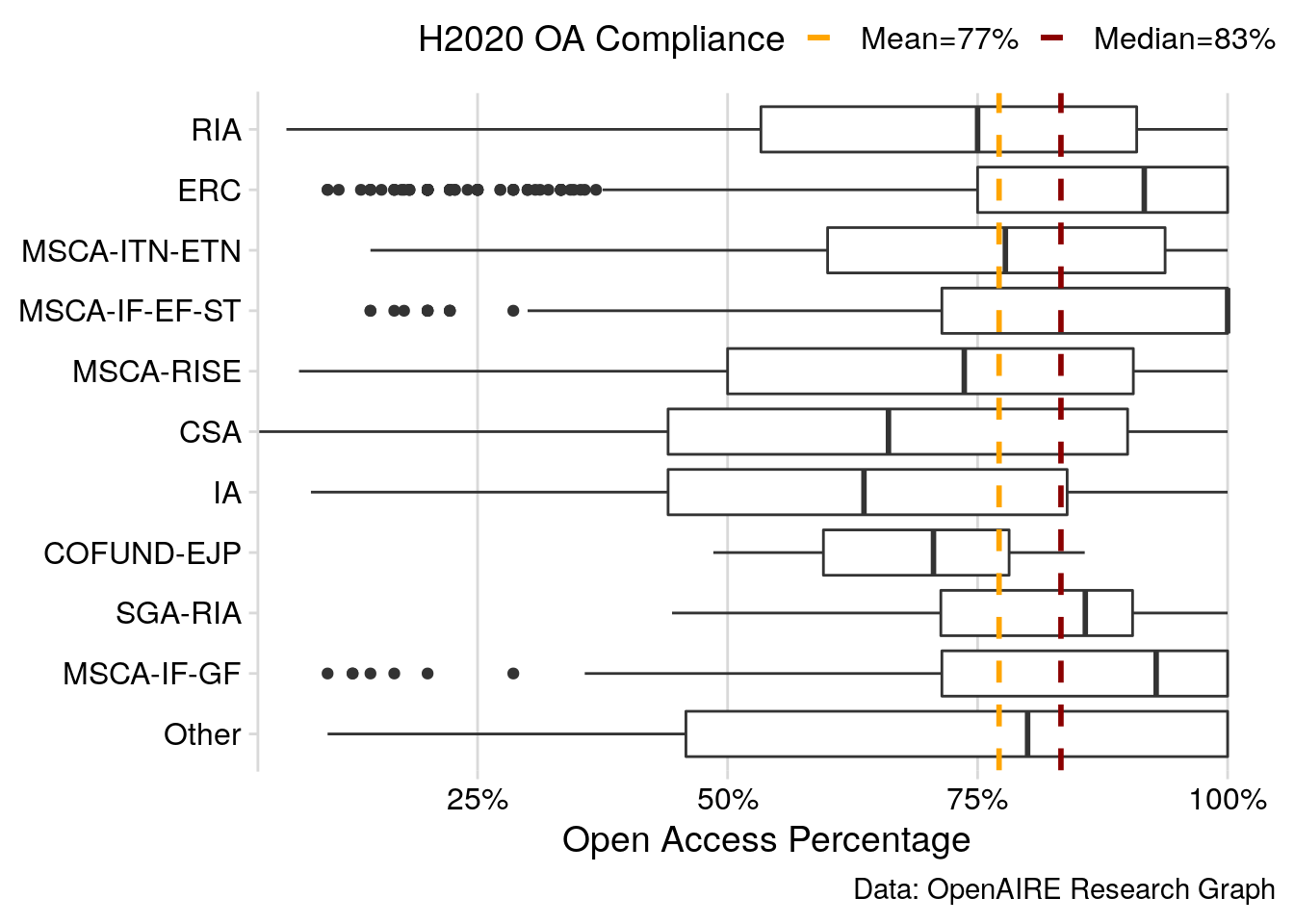
Figure 2: Open Access Compliance Rates of Horizon 2020 projects relative to funding activities, visualised as box plot. Only projects with at least five publications are shown individually.
About 77% of research publications under the H2020 open access mandate are openly available. Figure 2 highlights a generally high rate of compliance with the open access mandate, however, uptake levels vary the funding schemes. In particular, ERC grants and Marie Skłodowska-Curie activities show higher levels of compliance compared to the overall average.
Discussion and conclusion
Using data from the OpenAIRE Research Graph dumps makes it possible to put the results of a specific data analysis into context. Open access compliance rates of H2020 projects vary. These variations should be considered when reporting compliance rates of specific projects under the same open access mandate.
Although the OpenAIRE Research Graph is a large collection of scholarly data, it is likely that it still does not provide the whole picture. OpenAIRE mainly collects data from open sources. It is still unknown how the OpenAIRE Research Graph compares to well-established toll-access bibliometric data sources like the Web of Science in terms of coverage and data quality.
As a member of the OpenAIRE consortium, improving the re-use of the OpenAIRE Research Graph dumps has become a SUB Göttingen working priority. In the scholarly communication analysts team, we want to support this with a number of data analyses and outreach activities. In doing so, we will add more helper functions to the openairegraph R package. It targets data analysts and researchers who wish to conduct their own analysis using the OpenAIRE Research Graph, but are wary of handling its large data dumps.
If you like to contribute, head on over to the packages’ source code repository and get started!
Bengtsson, Henrik. 2020a. Future.apply: Apply Function to Elements in Parallel Using Futures. https://CRAN.R-project.org/package=future.apply.
———. 2020b. Future: Unified Parallel and Distributed Processing in R for Everyone. https://CRAN.R-project.org/package=future.
Hester, Jim, Gábor Csárdi, Hadley Wickham, Winston Chang, Martin Morgan, and Dan Tenenbaum. 2019. Remotes: R Package Installation from Remote Repositories, Including ’Github’. https://CRAN.R-project.org/package=remotes.
Larivière, Vincent, and Cassidy R. Sugimoto. 2018. “Do Authors Comply When Funders Enforce Open Access to Research?” Nature 562 (7728): 483–86. https://doi.org/10.1038/d41586-018-07101-w.
Manghi, Paolo, Claudio Atzori, Alessia Bardi, Jochen Schirrwagen, Harry Dimitropoulos, Sandro La Bruzzo, Ioannis Foufoulas, et al. 2019. “OpenAIRE Research Graph Dump.” Zenodo. https://doi.org/10.5281/zenodo.3516918.
Manghi, Paolo, Alessia Bardi, Claudio Atzori, Miriam Baglioni, Natalia Manola, Jochen Schirrwagen, and Pedro Principe. 2019. “The Openaire Research Graph Data Model.” Zenodo. https://doi.org/10.5281/zenodo.2643199.
Ooms, Jeroen. 2014. “The Jsonlite Package: A Practical and Consistent Mapping Between Json Data and R Objects.” arXiv:1403.2805 [stat.CO]. https://arxiv.org/abs/1403.2805.
Sievert, Carson. 2018. Plotly for R. https://plotly-r.com.
Wickham, Hadley, Mara Averick, Jennifer Bryan, Winston Chang, Lucy D’Agostino McGowan, Romain François, Garrett Grolemund, et al. 2019. “Welcome to the Tidyverse.” Journal of Open Source Software 4 (43): 1686. https://doi.org/10.21105/joss.01686.
Wickham, Hadley, Jim Hester, and Jeroen Ooms. 2019. Xml2: Parse Xml. https://CRAN.R-project.org/package=xml2.